Near Field and Far Field - Why Radio Changes with Distance
The Physics Behind Radio – Chapter 2
In the first chapter, we followed the idea of the electromagnetic wave
from Faraday’s field lines through Maxwell’s theory to Hertz’s
laboratory experiments. That story gave us the central picture: radio is
not sound in the air, and it is not a mysterious signal travelling
inside empty space without structure. It is an electromagnetic field
changing in time and propagating through space.
But this picture still hides an important question.
When does a changing electromagnetic field actually become a freely
travelling radio wave?
This sounds like a detail for antenna engineers, but it is one of the
most important distinctions in all of radio physics. Very close to a
source — a short dipole, a loop antenna, a transformer winding, a PCB trace, a charging coil or even a hand near an antenna — the electric and magnetic fields can still be strongly tied to the source that created
them. They may store energy locally, give it back during the next part
of the cycle, and react strongly to nearby objects.
Farther away, this complicated local structure gradually gives way to a
simpler travelling wave. In that region, the electric and magnetic
fields are locked together, their ratio approaches the wave impedance of
free space, and energy flows outward as radiation [1], [9].
This is the distinction between the near field and the far
field.
The near field is not “almost radio”. The far field is not “stronger
radio”. They are different regimes of the same Maxwell field. The
difference is not a matter of vocabulary, but of physics: local field
energy and coupling on one side, freely propagating radiation on the
other.
And there is a very practical way to feel this difference:
In the near field, a nearby object can become part of the transmitter’s
electromagnetic system.
In the far field, a receiver is usually only a listener.
That is why a hand close to a small antenna can detune a transmitter,
while a broadcast station does not care, in any practical sense, whether
one radio receiver or one million radio receivers are switched on.
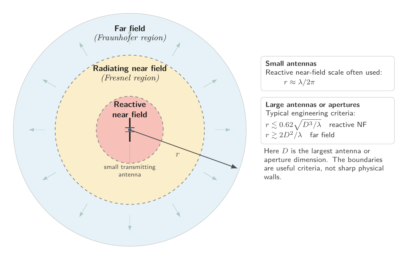
The Three Regions Around an Antenna
In everyday language we often speak of “the near field” and “the far
field” as if there were one clean border between them. In practice,
antenna theory usually divides the space around a radiating structure
into three regions:
- the reactive near field,
- the radiating near field, also called the Fresnel region,
- the far field, also called the Fraunhofer region [2], [6], [7].
The reactive near field is the region closest to the source. Here the fields are strongly influenced by the geometry of the antenna, the
current distribution, nearby conductors, dielectric materials, the human body, the housing of a device and even the feed cable. A large part of
the energy is not yet carried away permanently. Instead, it is stored
for part of the cycle in electric or magnetic form and then returned to
the source.
This is why a small change near an antenna can have a large effect. A hand, a metal plate, a nearby coil or a measurement probe does not merely “observe” the field. It can change the local field, alter the impedance seen by the transmitter and detune the system.
The radiating near field is already more wave-like, but it is still
not the clean far-field picture used in simple radio-link calculations.
Radiation is present, but the wavefront is still curved, and the field
pattern still changes with distance. This is the Fresnel region.
The far field is the region in which the radiation term dominates.
The local electric and magnetic fields are transverse to the direction
of propagation, they are essentially in phase, and their ratio
approaches the wave impedance of the medium. In free space this value is
approximately:
Z0 = E / H ≈ 376.73 Ω
This is not a resistor hidden in space. It is the ratio between electric
field strength and magnetic field strength for a freely propagating
electromagnetic wave in vacuum [9]. Once this relationship is
established, the field behaves locally like a travelling radio wave.
For electrically small antennas, a common practical rule places the
reactive near-field boundary roughly at:
r ≈ λ / 2π
where λ is the wavelength. This is a very useful rule of thumb, but it
is not a universal law of nature [1], [2]. It works best for small
radiators.
For large antennas, reflectors, horns, long Yagis and phased arrays, the
physical aperture size becomes just as important as the wavelength. A
common far-field criterion for large apertures is the Fraunhofer
distance:
r ≳ 2D² / λ
where D is the largest dimension of the antenna aperture [7]. This
explains why the far field of a large radar antenna, dish antenna or
phased array may begin much farther away than the simple λ/2π rule would
suggest.
This point matters in real radio work. A small handheld VHF antenna and
a large microwave dish may operate at very different scales, but both
obey the same field physics. The question is not simply: “How many
metres away am I?” The real question is: how large is the source
compared with the wavelength, and what approximation am I trying to use?
Why the Field Changes with Distance
The near-field/far-field distinction becomes clearer if we look at how
different parts of the electromagnetic field decrease with distance.
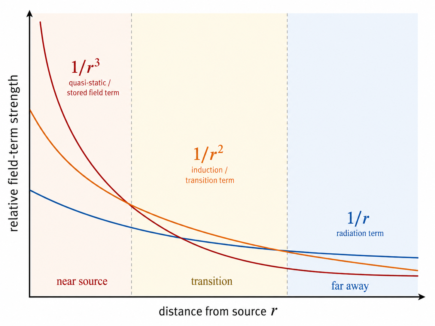
For localized, time-varying sources, the field can be described
qualitatively by terms that fall with distance like:
1/r³, 1/r² and 1/r
The 1/r³ term is associated with quasi-static near-field behaviour.
It is closely connected with local electric or magnetic energy storage.
The 1/r² term is often interpreted as an induction or transition
term. The 1/r term is the radiation term. Because 1/r decreases more
slowly than 1/r² or 1/r³, it eventually dominates at large distances.
That is why the far field is governed by radiation [3].
This also explains a familiar radio fact. In the far field, the field
amplitude falls approximately as 1/r, while the power density falls
approximately as 1/r². The power spreads over the surface of an
expanding sphere. Double the distance, and the same transmitted power is
distributed over four times the area.
But close to the source the picture is not so simple. The strong 1/r³
and 1/r² terms can dominate. Their presence means that nearby objects
can interact strongly with the source. A hand near a portable radio
antenna, a metal case around a transmitter, a nearby PCB ground plane,
or a coil placed close to another coil can all change the local field
and therefore the source behaviour itself.
That is the operational meaning of the reactive near field: the source
and its environment can still pull on each other electromagnetically.
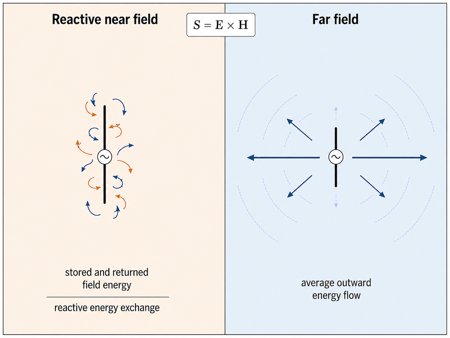
Energy That Leaves — and Energy That Comes Back
The Poynting vector describes the flow of electromagnetic energy. For real, time-dependent fields, its instantaneous form is:
S = E × H
It points in the direction in which electromagnetic energy flows. This
idea will become central in the next chapter, where we will look more
closely at where the energy in wires and transmission lines actually
travels. But it already helps us here.
In the far field, the time-averaged Poynting vector is mainly radial and
outward. Energy leaves the antenna and continues into space as
radiation. This is the regime of normal radio communication: a
transmitter launches power into the field, and a distant receiver
intercepts a tiny part of it [11], [22].
In the reactive near field, the instantaneous energy flow can be large,
but the time-averaged outward power may be small. Energy can slosh back
and forth between the source and the surrounding field. In circuit
language we would call this “reactive” behaviour. In field language it
means that the electric and magnetic energy storage near the source is
not simply the same thing as radiated power [4], [11].
This is why high field strengths near a coil, resonator or small antenna
do not automatically imply efficient radiation. A transformer can have
strong magnetic fields and transfer large power to a secondary winding,
while still being designed not to radiate significantly. A near-field
communication device can exchange data over a few centimetres without
acting like a miniature broadcast station. A wireless charger can
transfer useful power across a small gap while treating far-field
radiation mostly as an unwanted loss [12], [14], [15].
The near field is therefore not a failed far field. It is a useful
physical regime in its own right.
When the Receiver Is Part of the System
This gives us a very intuitive way to understand the difference between
near-field coupling and far-field reception.
In the reactive near field, a nearby object can become part of the
transmitter’s electromagnetic system. A receiving coil, a hand, a metal
enclosure or another antenna can change the local field, alter the
antenna impedance and even detune the source. The field has not yet
fully separated from the structure that created it.
A transformer is the most obvious example. The secondary winding is not
just “receiving a wave”. It is magnetically coupled to the primary
winding. If the secondary load changes, the primary side sees that
change. The receiver becomes part of the coupled electromagnetic system
[12].
The same is true, in a looser form, for NFC, RFID and inductive
charging. The reader coil and the tag or receiver coil are close enough
that their fields overlap strongly. Energy can be transferred
efficiently because the two systems are coupled through the near field
[13], [14], [15].
In the far field, the situation is different. The transmitter has
already launched energy into a freely propagating wave. A receiver can
absorb a tiny part of that wave, but it normally does not behave like an
additional load connected back to the transmitter. This is why a
broadcast transmitter does not care, in any practical sense, whether one
radio receiver or one million radio receivers are listening. The
receivers take energy from the already radiated field; they do not
significantly pull energy back through the transmitter.
Of course, this is not an absolute rule. A large reflector, an aircraft,
a wall or a large absorbing structure in the far field can scatter or
reflect energy back toward the transmitter. Radar is based on exactly
such returned radiation. But this is a delayed wave interaction. The
reflected field must travel back to the transmitter. It is not the
immediate source-field coupling that characterizes the reactive near
field.
A useful short version is:
In the near field, a receiver can be part of the transmitter’s load.
In the far field, a receiver is normally just a listener to energy that
has already escaped.
That sentence captures much of the physics.
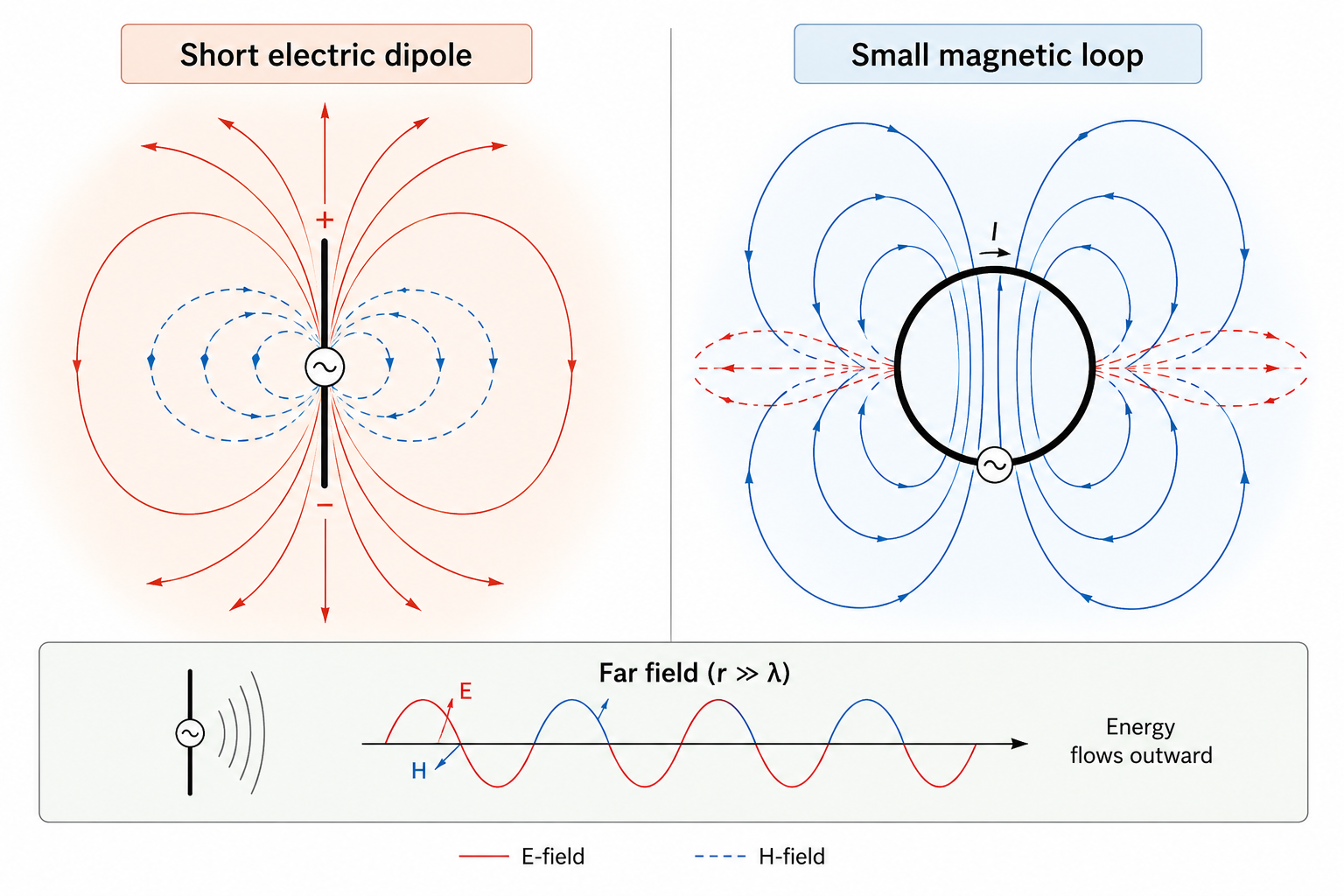
Electric Near Field and Magnetic Near Field
A common misunderstanding is that near field means magnetic field, while
far field means electromagnetic wave. That is too simple.
The character of the near field depends strongly on the source.
A short electric dipole is the classic example of an electrically
dominated near field. Charges accumulate at the ends of the conductor,
and the nearby field is strongly related to this changing charge
separation. In the near field the ratio E/H is high. The field behaves
in a largely capacitive way.
A small loop is the opposite archetype. Its current circulates around an
area and produces a strong local magnetic flux. The nearby field is
therefore magnetically dominated. In the near field the ratio E/H is
low. The field behaves in a largely inductive way [1], [10].
For a short electric dipole, the near-field wave impedance is often
approximated as being proportional to:
E/H ≈ 60 λ/r Ω
For a small magnetic loop, the corresponding near-field behaviour is
roughly:
E/H ≈ 2370 r/λ Ω
These expressions should not be read as universal antenna laws for every
geometry. Their purpose is to show the trend. The electrically short
dipole has a high near-field impedance; the small loop has a low
near-field impedance. As distance increases, both tend toward the
free-space value of about 377 Ω [1], [9].
This is a beautiful result. In the far field, the initial asymmetry
largely disappears. Whether the antenna began as an electric dipole or a
magnetic loop, the radiated wave eventually becomes an electromagnetic
wave with electric and magnetic fields locked together.
The source still matters for radiation pattern, efficiency and
polarization. But locally, in the far field, the wave is no longer
“mostly electric” or “mostly magnetic”. It is both.
Low Frequency Does Not Automatically Mean Magnetic Field
Another common shortcut is the statement: “At low frequencies, the
magnetic field dominates.”
This is not generally correct.
What is true is that low frequency means long wavelength. A longer
wavelength makes the region r ≲ λ/2π larger in metres. At 100 kHz, the
wavelength is about 3 km, and λ/2π is roughly 477 m. At 2.4 GHz, the
wavelength is about 12.5 cm, and λ/2π is only about 2 cm.
So low frequency often makes quasi-static thinking useful over larger
distances. But it does not decide whether the near field is mainly
electric or magnetic. That depends primarily on the source geometry. A
small electric structure remains electrically dominated in its near
field. A small loop remains magnetically dominated in its near field, as
long as it is small compared with the wavelength [1].
The frequency sets the scale. The source sets the character.
| Frequency | Wavelength λ | λ/2π | Practical meaning |
|---|---|---|---|
| 100 kHz | 2997.9 m | 477.1 m | Quasi-static near-field thinking can extend over hundreds of metres for small sources. |
| 1 MHz | 299.8 m | 47.7 m | The near-field scale is still large; induction effects can remain important. |
| 100 MHz | 2.998 m | 0.477 m | For small VHF antennas, the reactive near field is on the order of decimetres. |
| 2.4 GHz | 0.1249 m | 0.0199 m | For small WLAN/Bluetooth antennas, the λ/2π scale is only about 2 cm. |
The table uses:
λ = c / f
with:
c = 299,792,458 m/s
the defined speed of light in vacuum [20].
The practical lesson is simple: the near field does not vanish at high
frequency, and it does not become automatically magnetic at low
frequency. It changes scale.
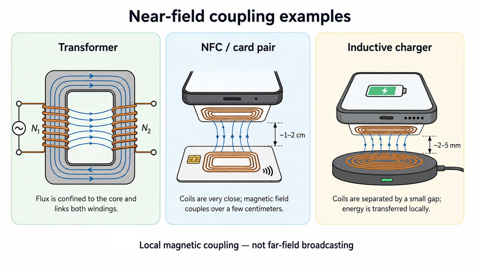
Transformers, motors, NFC and wireless charging
The transformer is the cleanest everyday reminder that electromagnetic energy
transfer does not automatically mean far-field radio. A changing current in the
primary winding creates a changing magnetic flux, usually guided through an
iron or ferrite core. This flux links the secondary winding and induces a voltage
there. The secondary is not merely “receiving a wave”; it is part of a coupled
near-field system [12].
The same family of ideas appears in induction motors, NFC, HF RFID and
wireless chargers. NFC operates at 13.56 MHz, where the wavelength is about
22 m and λ/2π is about 3.5 m. A phone and a contactless card separated by a few
centimetres are therefore deep in the reactive near field. A Qi charger also uses
close magnetic coupling between coils, often with resonance, rather than using
ordinary far-field radiation as its useful channel [14], [15].
This chapter only needs the distinction: near-field systems couple locally and can
load each other; far-field radio launches energy that then travels independently.
Chapter 6 will return to transformers, motors, NFC and wireless charging in more
detail and explain why these systems can transfer energy efficiently while hardly
radiating.
Antennas, Apertures and the Problem of “Far Enough”
Small antennas make the near-field/far-field story easy to introduce.
Large antennas make it more interesting.
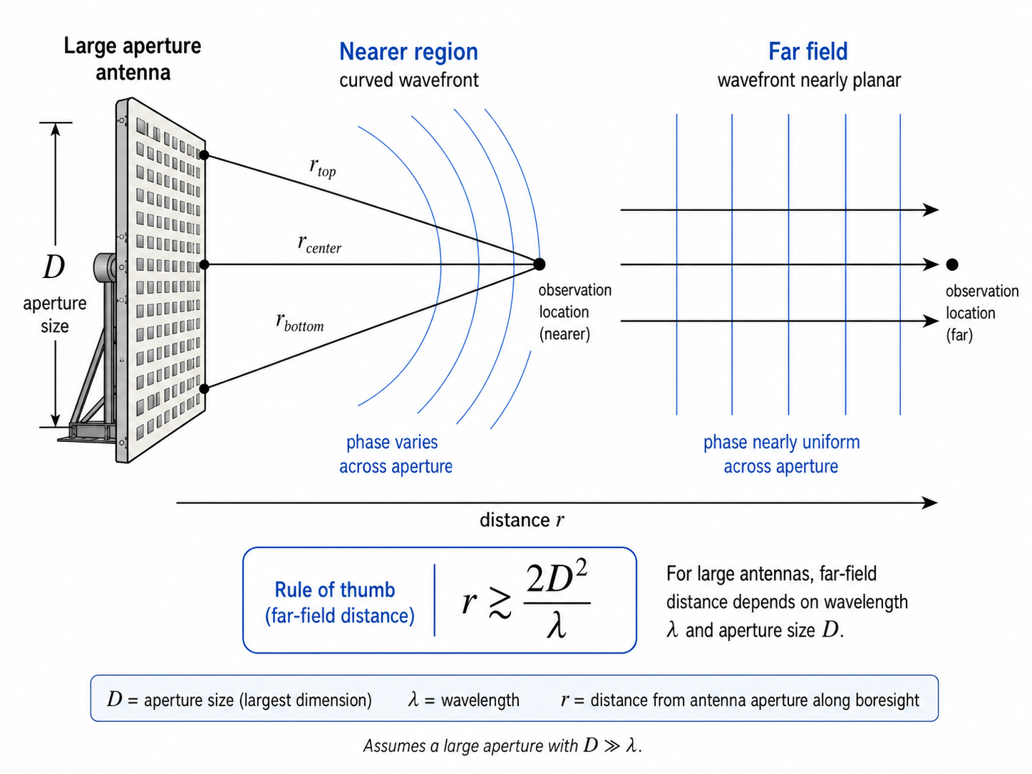
A short dipole or small loop can often be discussed using the λ/2π rule
for the reactive near field. But large antennas have an additional
problem: the wavefront must become sufficiently flat across the whole
aperture. If the antenna has a large physical size D, then different
parts of the aperture see slightly different path lengths to the
observation point. These path differences create phase differences. Only
when those phase errors become small enough does the far-field
approximation become valid [7].
That is why the Fraunhofer distance contains D²:
r ≳ 2D² / λ
This is not just theoretical bookkeeping. It affects antenna
measurements. If a large dish, horn, radar antenna or phased array must
be measured in the true far field, the required range length may become
impractically large. Instead, engineers often measure the field much
closer to the antenna on a plane, cylinder or sphere, and then
mathematically transform the measured near field into a far-field
radiation pattern. This is called near-field to far-field transformation
[6], [16].
Modern communication research has made this issue newly important. Large
antenna arrays for millimetre-wave, sub-THz and proposed 6G systems can
be so physically large in wavelengths that users may be many wavelengths
away and still not be in the classical far field of the whole array. In
such systems, one sometimes has to treat the wavefront as spherical
rather than plane, and near-field beamforming becomes a real system
design topic rather than a textbook curiosity [8], [21].
Radio amateurs know a simpler version of the same lesson. A small
handheld antenna, a long Yagi, a dish feed and a parabolic reflector do
not all “settle” into their far-field behaviour at the same physical
distance. The wavelength matters, but the antenna size matters too.
Transmission Lines Are Not Supposed to Radiate
There is one more important case: wires that are meant to guide
electromagnetic energy rather than radiate it.
An ideal coaxial cable confines the electromagnetic field mainly to the
dielectric region between the inner conductor and the inside of the
shield. The energy is guided along the cable by the field structure.
Outside the shield, the fields ideally cancel. A balanced two-wire line
works differently, but it also relies on symmetry: equal and opposite
currents produce fields that largely cancel in the far field when the
line is well balanced [11].
When this symmetry is broken, the line can become an unwanted antenna.
Common-mode currents on a coaxial cable, abrupt geometry changes, poor
shielding, poor grounding or unbalanced transitions can all turn a feed
line into part of the radiator.
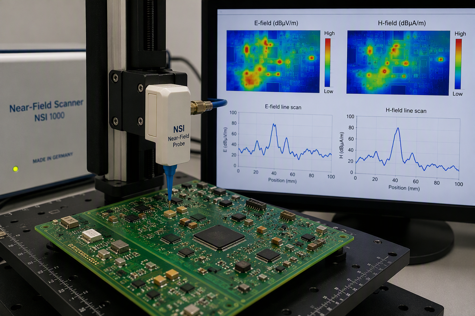
This is why near-field thinking is also essential in EMC work. Engineers
use small E-field and H-field probes to scan PCBs, cables and integrated
circuits at millimetre distances. They are not trying to measure a clean
far-field radiation pattern. They are looking for local field sources,
coupling paths and hot spots [16].
A near-field probe is almost the opposite of a distant receiving
antenna. The distant antenna asks: “What wave has finally escaped?” The
near-field probe asks: “What local field is being created here, before
it becomes a system-level radiation problem?”
Human Exposure and the Limits of Simple Power Density
The near-field/far-field distinction also matters in exposure
assessment.
In the far field, it is often meaningful to think in terms of power
density in free space. The wave is locally well formed, E and H have a
fixed ratio, and simple relationships can be used to estimate the field.
Close to a body-worn or handheld transmitter, this simplification can
fail. The body is not merely a passive object sitting in a plane wave.
It can interact with the local field, absorb energy in a
geometry-dependent way, and change the source environment. This is why
specific absorption rate, or SAR, becomes important for devices used
close to the body [17].
The same transmitted power can lead to different local absorption
depending on antenna position, frequency, body geometry and field
distribution. This is another reminder that “near” and “far” are not
just distances. They describe whether the field can be treated as a
freely propagating wave or whether the local source-field-object
interaction still matters.
Historical Roots: Faraday, Maxwell and Hertz
The near-field/far-field distinction is a later technical refinement,
but its roots go back to the birth of field theory.
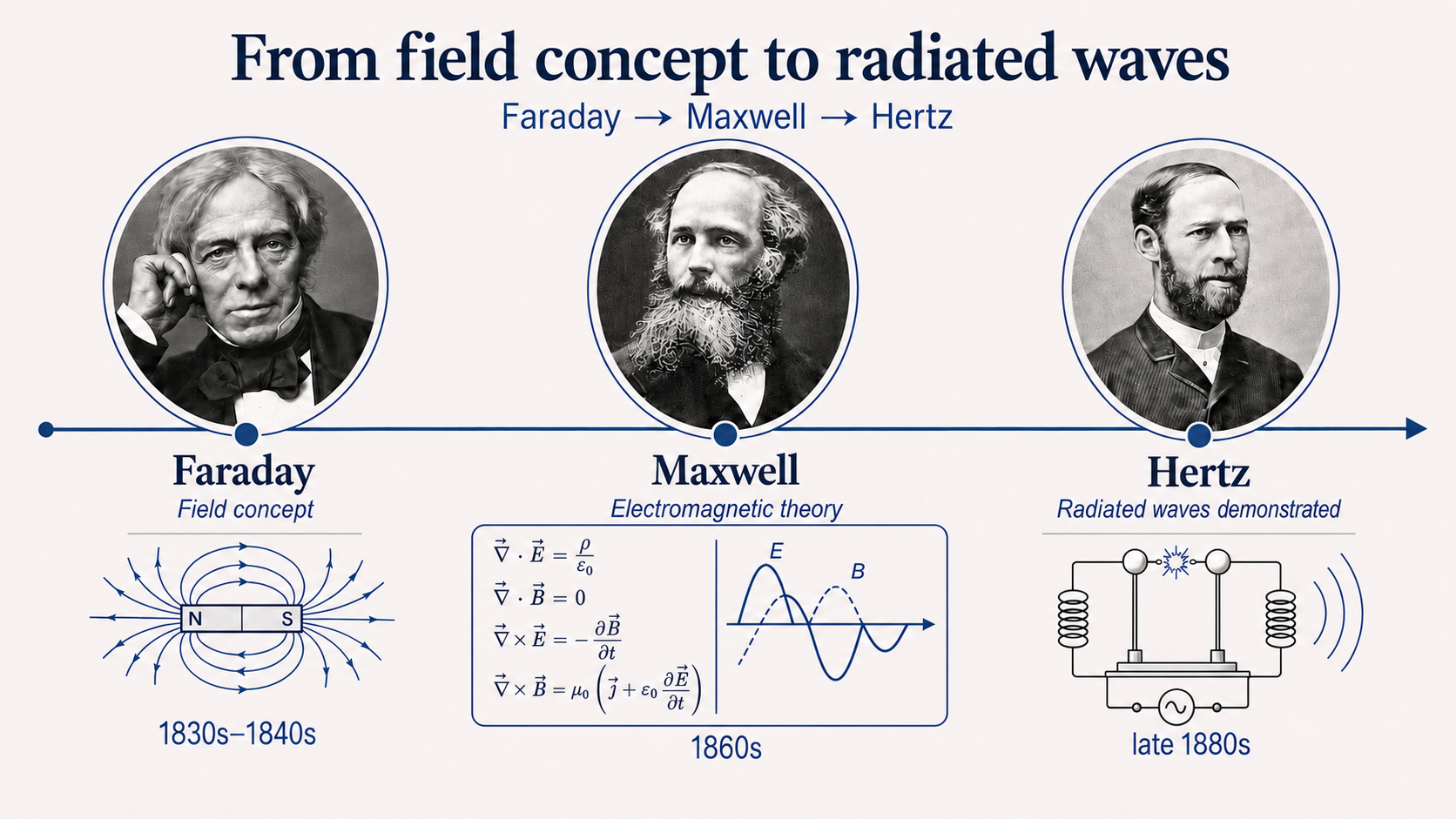
Michael Faraday did not write Maxwell’s equations, but he changed the
way physicists imagined electrical and magnetic action. His field-line
picture replaced the older idea of instantaneous action at a distance
with the idea that something physically meaningful exists in the space
around charges, currents and magnets [5].
James Clerk Maxwell turned this field intuition into a mathematical
theory. In his work on physical lines of force and in “A Dynamical
Theory of the Electromagnetic Field”, Maxwell showed that electricity,
magnetism and light belonged to one unified framework. His equations
predicted waves travelling at the speed of light. Light itself became an
electromagnetic phenomenon [18].
Heinrich Hertz then demonstrated electromagnetic waves experimentally.
His spark-gap transmitters and resonators showed reflection, refraction,
interference and polarization — the same optical-like properties
expected from Maxwell’s theory [19].
From today’s perspective, Hertz’s experiments are especially interesting
because they contain both worlds. Close to his apparatus there were
strong local fields, coupling and resonance. Farther away there was
radiated energy behaving like a wave. Later radio engineering turned
this into a practical distinction: near-field coupling on one side,
far-field radiation on the other.
Common Misunderstandings
Several persistent misunderstandings become easier to correct once the
near-field/far-field distinction is clear.
The first is: “Every electromagnetic field is already a radio
wave.”
Not really. Close to a time-varying source there can be strong reactive
field components that should not be described as a freely propagating
wave. The far field is the region where the radiation term dominates
[1], [3].
The second is: “The magnetic field dominates at low frequency.”
Frequency changes the wavelength and therefore the physical scale of the
near field. But electric or magnetic dominance depends mainly on the
source. A short dipole and a small loop do not have the same near field
[1], [10].
The third is: “The near field ends at one exact distance.”
No. The common boundaries are engineering criteria. They depend on
wavelength, antenna size, acceptable phase error, observation angle and
application. The λ/2π rule is useful for small antennas; the Fraunhofer
distance is more appropriate for large apertures [2], [7], [8],
[22].
The fourth is: “Wireless power and radio communication are the same
mechanism.”
Only in the broad sense that both are electromagnetic. Inductive
charging and NFC use local near-field coupling. Broadcasting, satellite
links and normal radio communication use far-field radiation [14],
[15].
The fifth is: “In the far field there is either an electric field or a
magnetic field.”
No. In the far field the two are inseparable parts of the travelling
electromagnetic wave. They are transverse, in phase, and related by the
wave impedance of the medium [9].
The sixth is: “A transmitter must work harder when more receivers are
listening.”
For ordinary far-field radio reception, no. A distant receiver absorbs
only a tiny part of an already radiated wave. Adding more normal
receivers does not significantly change the transmitter’s load. This is
very different from the near field, where a nearby coil, antenna or
object can couple back into the source and change its impedance [1],
[11], [12].
Why This Matters for Radio
Radio technology lives from the controlled transition between local
fields and radiated waves.
A transformer tries to keep energy in a local magnetic coupling path. A
coaxial cable tries to guide the field without letting it escape. An
antenna is designed to do the opposite: it converts guided or localized
electromagnetic energy into radiation. A near-field probe deliberately
samples the messy local field before it becomes a clean far-field
pattern. A far-field antenna measurement tries to observe the final
radiated wave after the local complications have died away.
This is why antennas are subtle devices. They are not magic metal rods
that “throw electrons into space”. They are structures that shape
electric and magnetic fields so that some of the energy no longer
returns to the source, but continues outward as radiation.
In the near field, the source still matters intimately. A receiver, a
hand, a metal plate or a nearby resonator can become part of the same
coupled system.
In the far field, the wave has become independent enough to travel. It
no longer asks whether anyone is listening.
That is the quiet boundary at the heart of radio.
Sources and further reading
[1] Near and far field
https://en.wikipedia.org/wiki/Near_and_far_field
[2] Nahfeld und Fernfeld (Antennen)
https://de.wikipedia.org/wiki/Nahfeld_und_Fernfeld_(Antennen)
[3] Jefimenko’s equations
https://en.wikipedia.org/wiki/Jefimenko's_equations
[4] Evanescent field
https://en.wikipedia.org/wiki/Evanescent_field
[5] Michael Faraday
https://en.wikipedia.org/wiki/Michael_Faraday
[6] Antenna measurement
https://en.wikipedia.org/wiki/Antenna_measurement
[7] Fraunhofer distance
https://en.wikipedia.org/wiki/Fraunhofer_distance
[8] Emil Björnson, Özlem Tuğfe Demir, Luca Sanguinetti, “A Primer on
Near-Field Beamforming for Arrays and Reconfigurable Intelligent
Surfaces”
https://arxiv.org/abs/2110.06661
[9] Wellenwiderstand des Vakuums
https://de.wikipedia.org/wiki/Wellenwiderstand_des_Vakuums
[10] Loop antenna
https://en.wikipedia.org/wiki/Loop_antenna
[11] Poynting vector
https://en.wikipedia.org/wiki/Poynting_vector
[12] Transformer
https://en.wikipedia.org/wiki/Transformer
[13] Induction motor
https://en.wikipedia.org/wiki/Induction_motor
[14] Near-field communication
https://en.wikipedia.org/wiki/Near-field_communication
[15] Qi standard
https://en.wikipedia.org/wiki/Qi_(standard)
[16] Near-field scanner
https://en.wikipedia.org/wiki/Near-field_scanner
[17] Specific absorption rate
https://en.wikipedia.org/wiki/Specific_absorption_rate
[18] A Dynamical Theory of the Electromagnetic Field
https://en.wikipedia.org/wiki/A_Dynamical_Theory_of_the_Electromagnetic_Field
[19] Heinrich Hertz
https://en.wikipedia.org/wiki/Heinrich_Hertz
[20] CODATA Recommended Values of the Fundamental Physical Constants:
2022
https://arxiv.org/abs/2409.03787
[21] Mehdi Monemi et al., “A Study on Characterization of Near-Field
Sub-Regions For Phased-Array Antennas”
https://arxiv.org/abs/2411.02425
[22] J. David Jackson, “How an antenna launches its input power into
radiation: the pattern of the Poynting vector at and near an antenna”
https://arxiv.org/abs/physics/0506053